1
2
3
4
5
6
7
8
9
10
11
12
13
14
15
16
17
18
19
20
21
22
23
24
25
26
27
28
29
30
31
32
33
34
35
36
37
38
39
40
41
42
43
44
45
46
47
48
49
50
51
52
53
54
55
56
57
58
59
60
61
62
63
64
65
66
67
68
69
70
71
72
73
74
75
76
77
78
79
80
81
82
83
84
85
86
87
88
89
90
91
92
93
94
95
96
97
98
99
100
101
102
103
104
105
106
107
108
109
110
111
112
113
114
115
116
117
118
119
120
121
122
123
124
125
126
127
128
129
130
131
132
133
134
135
136
137
138
139
140
141
142
|
clc
clear all
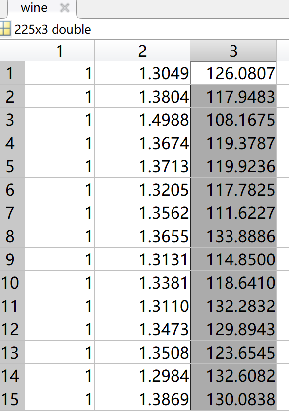
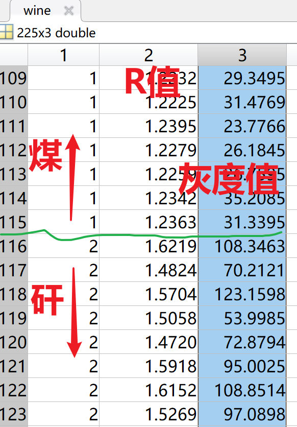
load wine.mat;
data1 = wine(1:115,:);
data2 = wine(116:225,:);
p = 2;
q = p+1;
data0=[data1;data2];
train_data=data0(:,p:q);
train_label=data0(:,1);
[train_data,pstrain] = mapminmax(train_data');
pstrain.ymin = 0;
pstrain.ymax = 1;
[train_data,pstrain] = mapminmax(train_data,pstrain);
train_data =train_data';
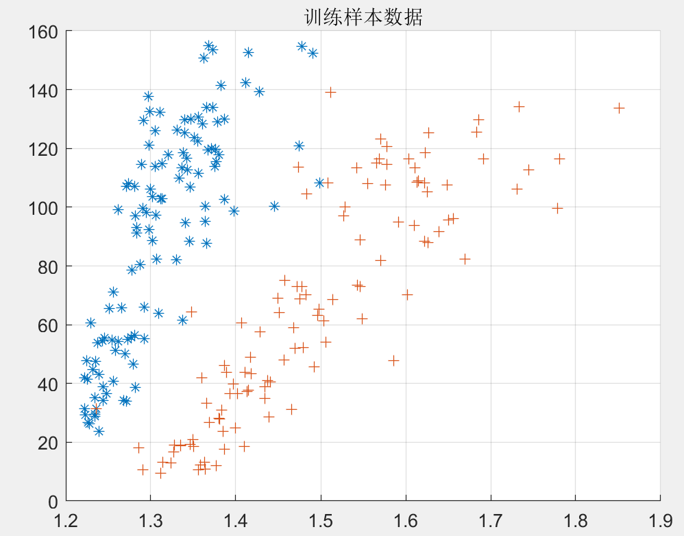
figure('NumberTitle', 'on', 'Name','灰度均值与灰度方差');
hold on;
grid on;
plot(data1(:,p),data1(:,q),'*'),
plot(data2(:,p),data2(:,q),'+'),
title('训练样本数据');
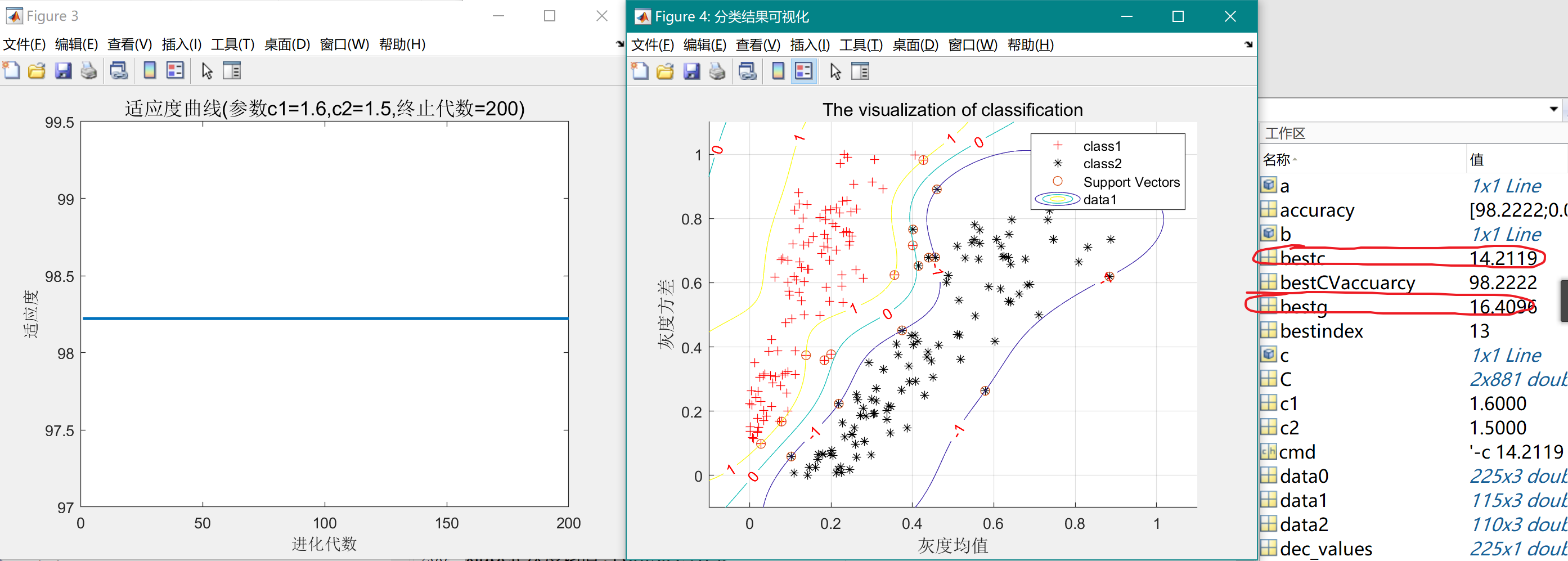
c1 = 1.6;
c2 = 1.5;
maxgen=200;
sizepop=30;
popcmax=10^(2);
popcmin=10^(-1);
popgmax=10^(3);
popgmin=10^(-2);
k = 0.6;
Vcmax = k*popcmax;
Vcmin = -Vcmax ;
Vgmax = k*popgmax;
Vgmin = -Vgmax ;
v = 3;
for i=1:sizepop
pop(i,1) = (popcmax-popcmin)*rand+popcmin;
pop(i,2) = (popgmax-popgmin)*rand+popgmin;
V(i,1)=Vcmax*rands(1);
V(i,2)=Vgmax*rands(1);
cmd = ['-v ',num2str(v),' -c ',num2str( pop(i,1) ),' -g ',num2str( pop(i,2) )];
fitness(i) = libsvmtrain(train_label,train_data, cmd);
fitness(i) = -fitness(i);
end
[global_fitness,bestindex]=min(fitness);
local_fitness=fitness;
global_x=pop(bestindex,:);
local_x=pop;
tic
for i=1:maxgen
for j=1:sizepop
wV = 0.9;
V(j,:) = wV*V(j,:) + c1*rand*(local_x(j,:) - pop(j,:)) + c2*rand*(global_x - pop(j,:));
if V(j,1) > Vcmax
V(j,1) = Vcmax;
end
if V(j,1) < Vcmin
V(j,1) = Vcmin;
end
if V(j,2) > Vgmax
V(j,2) = Vgmax;
end
if V(j,2) < Vgmin
V(j,2) = Vgmin;
end
wP = 0.6;
pop(j,:)=pop(j,:)+wP*V(j,:);
if pop(j,1) > popcmax
pop(j,1) = popcmax;
end
if pop(j,1) < popcmin
pop(j,1) = popcmin;
end
if pop(j,2) > popgmax
pop(j,2) = popgmax;
end
if pop(j,2) < popgmin
pop(j,2) = popgmin;
end
if rand>0.5
k=ceil(2*rand);
if k == 1
pop(j,k) = (20-1)*rand+1;
end
if k == 2
pop(j,k) = (popgmax-popgmin)*rand+popgmin;
end
end
cmd = ['-v ',num2str(v),' -c ',num2str( pop(j,1) ),' -g ',num2str( pop(j,2) )];
fitness(j) = libsvmtrain(train_label,train_data, cmd);
fitness(j) = -fitness(j);
end
if fitness(j) < local_fitness(j)
local_x(j,:) = pop(j,:);
local_fitness(j) = fitness(j);
end
if fitness(j) < global_fitness
global_x = pop(j,:);
global_fitness = fitness(j);
end
fit_gen(i)=global_fitness;
end
toc
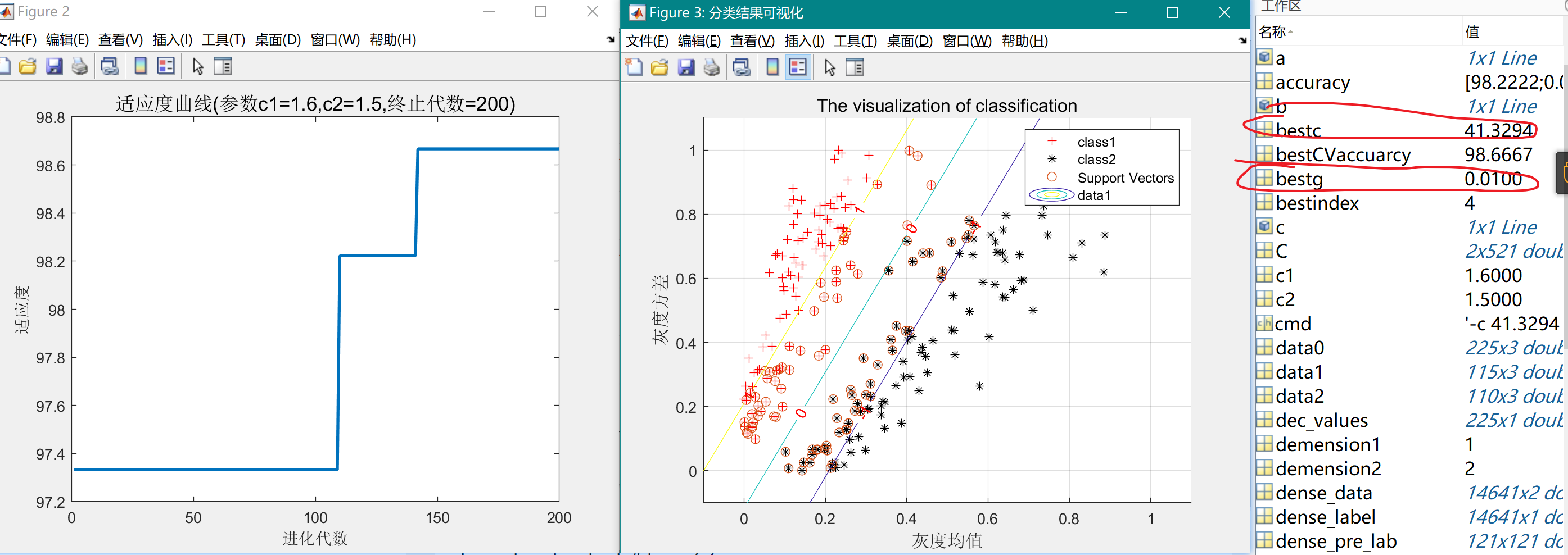
figure,
plot(-fit_gen,'LineWidth',2);
title(['适应度曲线','(参数c1=',num2str(c1),',c2=',num2str(c2),',终止代数=',num2str(maxgen),')'],'FontSize',13);
xlabel('进化代数');ylabel('适应度');
bestc = global_x(1)
bestg = global_x(2)
bestCVaccuarcy = -fit_gen(maxgen);
cmd = ['-c ',num2str( bestc ),' -g ',num2str( bestg )];
|