分水岭算法理解与MATLAB实例分析
如下图所示:
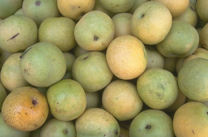
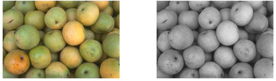
苹果与苹果之间均有粘连,如果使用大津法做图像分割,则会将粘连的多个苹果分割为一个。
分水岭算法将图像看作一个拓扑地形图,其中灰度值被认为是地形高度值。高灰度值对应着山峰,低灰度值对应着山谷。
如下图所示(原图像):
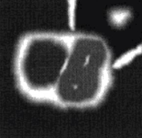
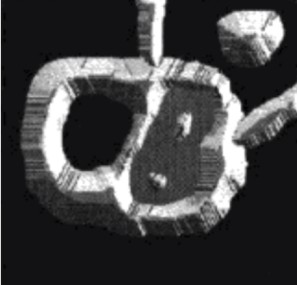
将原图像进行处理转化为地形俯视图:
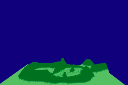
地形图三维视图:
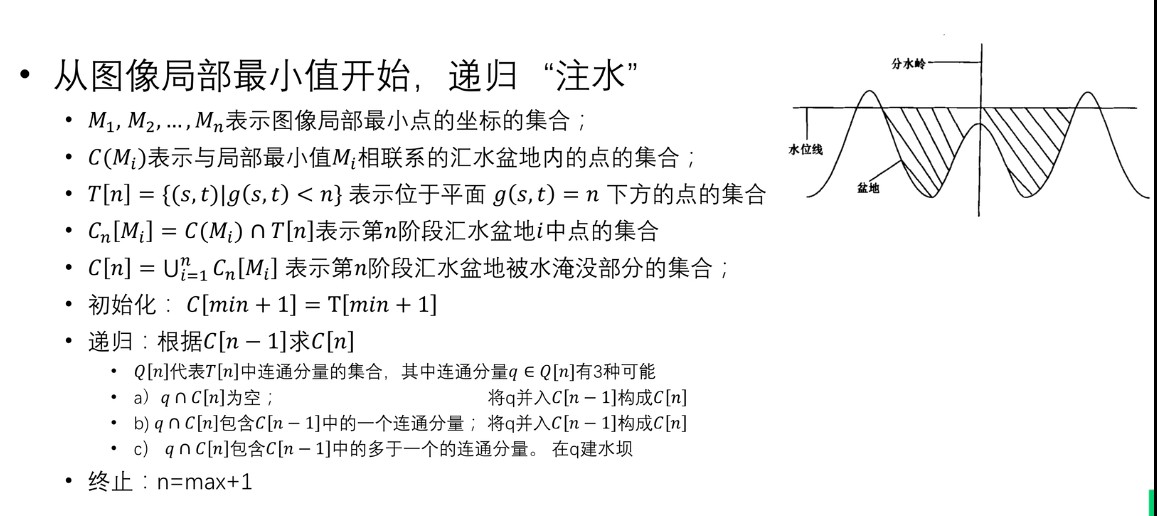
将水从任一处留下来,它会朝地势较低的地方流动,直到某一局部低洼处才停下来。这个低洼处被称为吸水盆地。最终所有的水都会聚集在不同的吸水盆地。
吸水盆地之间的山脊被称为分水岭。
水从分水岭留下时,它朝不同吸水盆地流去的可能性相同。
- 最小值点:水最终汇集的地方;
- 盆地边缘点:水会等概率的流向任何盆地;
- 盆地其他点:水会聚集到局部最小点。
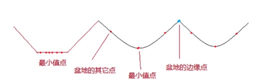
上图中红色的点可以视作注水口。
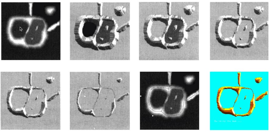
假设我们在盆地的最小值点打一个洞,然后往盆地里面注水,并且阻止两个盆地的水汇集,并在两个盆地的水汇集的时刻,在交界线的边缘上(也即分水岭线),建立一个水坝,来阻止两个盆地的水汇集成一片水域。
这样图像就被分成2个像素集,一个是注水盆地像素集,一个是分水岭线像素集。
对应到图像分割,就是要在灰度图像中找到不同的吸水盆地和分水岭。
不同的吸水盆地和分水岭组成的区域即为我们要分割的目标。
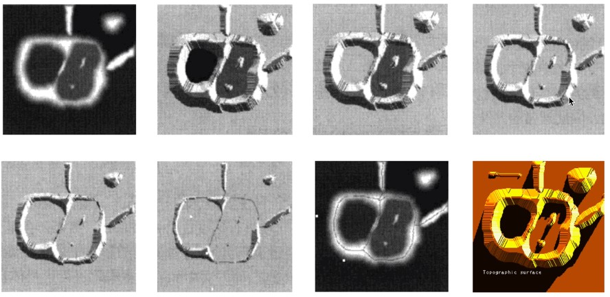
逐渐漫水过程示意图:
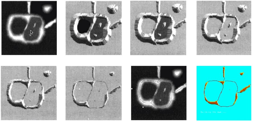
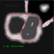
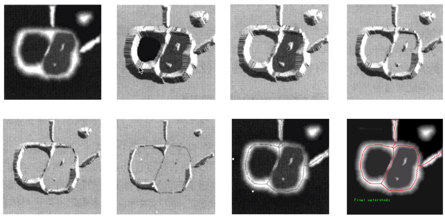
最终我们想要的结果:
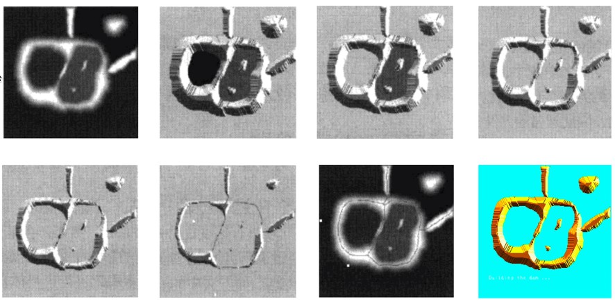
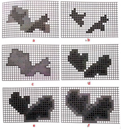
水坝的构建
- 在实际操作中,水位的上升常利用灰度0~255的分层处理来实现,当处理到第N层时,灰度小于N的像素就会被淹没。
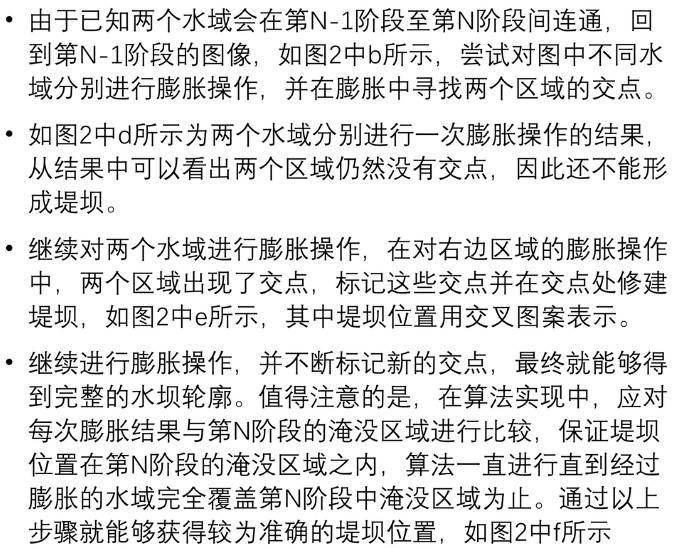
- 图中a显示了两个相邻聚水盆,其中颜色越深的区域海拔越低。
- 当水位逐渐上升到第N-1阶段时,黑色区域首先被淹没。
- 借助膨胀的方法,在水域之间适当的位置构建堤坝防止水域的连通。
分水岭算法实现步骤:
分水岭算法的实现
在MATLAB中,函数watershed()即为分水岭函数。L = watershed(A),L是一个标记矩阵,标记分水岭算法分割出的各“分水岭”区域。
1
2
3
4
| rgb = imread('pears.png');
I = rgb2gray(rgb);
subplot(121),imshow(rgb);
subplot(122),imshow(I);
|
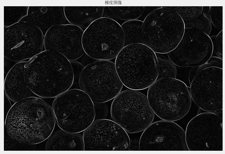
为了更加突出边缘信息,针对梯度图像进行处理:
1
2
3
4
5
6
|
hy = fspecial('sobel');hx = hy';
Iy = imfilter(double(I),hy,'replicate');
Ix = imfilter(double(I),hx,'replicate');
gradmag = sqrt(Ix.^2 + Iy.^2);
figure(2),imshow(gradmag,[]),title('梯度幅值图像');
|
接下来使用梯度幅值图像做分水岭:
1
2
3
4
|
L = watershed(gradmag);
Lrgb = label2rgb(L);
figure(3),imshow(Lrgb),title('梯度幅值图像做分水岭');
|
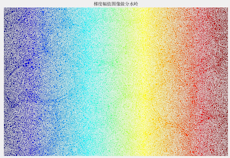
结果图像过分割太严重(寻找到的局部极小值太多),接下来需要对其进行改进,首先标注,然后分割,即把较多的极小值点进行合并。
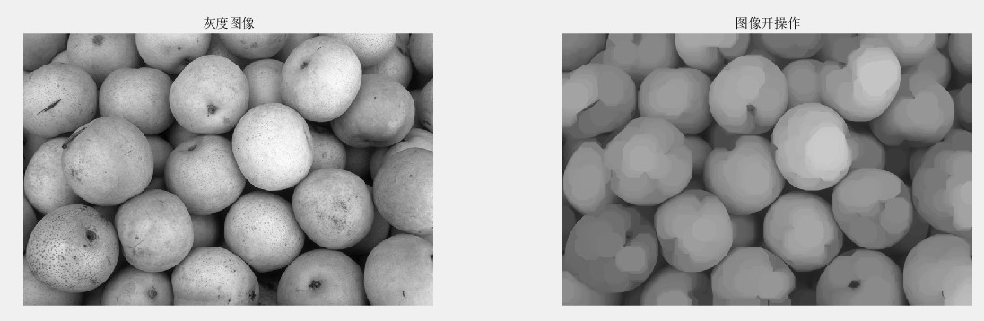
事前标记(Mark)目标部分区域(运用形态学中的开闭运算),在这个区域的水淹没过程中,水平面都是从定义的高度开始的,这样可以避免一些很小的噪声极值区域的分割。
1
2
3
4
5
6
7
8
|
se = strel('disk', 20);
Io = imopen(I, se);
figure('units', 'normalized', 'position', [0 0 1 1]);
subplot(1, 2, 1); imshow(I, []); title('灰度图像');
subplot(1, 2, 2); imshow(Io), title('图像开操作')
|
1
2
3
4
5
6
|
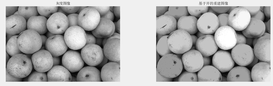
Ie = imerode(I, se);
Iobr = imreconstruct(Ie, I);
figure('units', 'normalized', 'position', [0 0 1 1]);
subplot(1, 2, 1); imshow(I, []); title('灰度图像');
subplot(1, 2, 2); imshow(Iobr, []), title('基于开的重建图像')
|
1
2
3
4
5
6
7
8
|
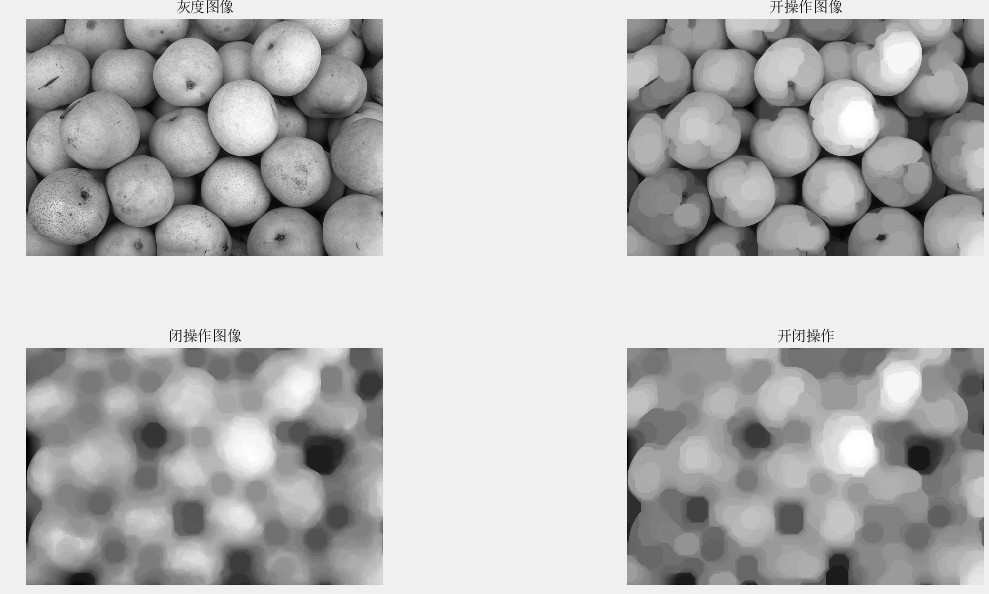
Ioc = imclose(Io, se);
Ic = imclose(I, se);
figure('units', 'normalized', 'position', [0 0 1 1]);
subplot(2, 2, 1); imshow(I, []); title('灰度图像');
subplot(2, 2, 2); imshow(Io, []); title('开操作图像');
subplot(2, 2, 3); imshow(Ic, []); title('闭操作图像');
subplot(2, 2, 4); imshow(Ioc, []), title('开闭操作');
|
1
2
3
4
5
6
7
8
9
|
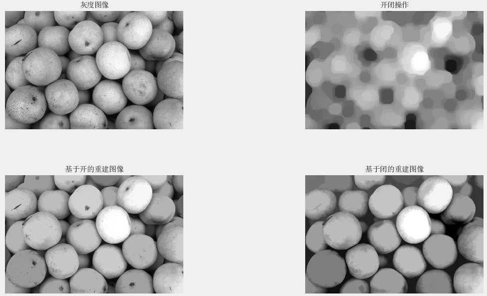
Iobrd = imdilate(Iobr, se);
Iobrcbr = imreconstruct(imcomplement(Iobrd), imcomplement(Iobr));
Iobrcbr = imcomplement(Iobrcbr);
figure('units', 'normalized', 'position', [0 0 1 1]);
subplot(2, 2, 1); imshow(I, []); title('灰度图像');
subplot(2, 2, 2); imshow(Ioc, []); title('开闭操作');
subplot(2, 2, 3); imshow(Iobr, []); title('基于开的重建图像');
subplot(2, 2, 4); imshow(Iobrcbr, []), title('基于闭的重建图像');
|
1
2
3
4
5
6
|
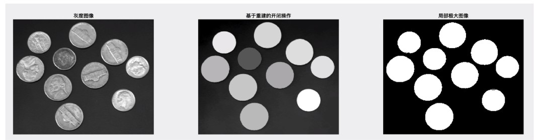
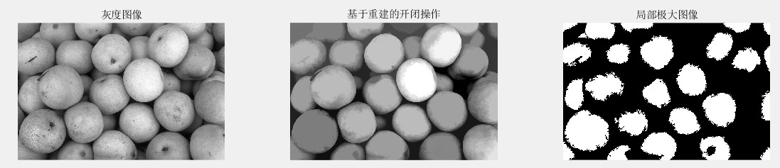
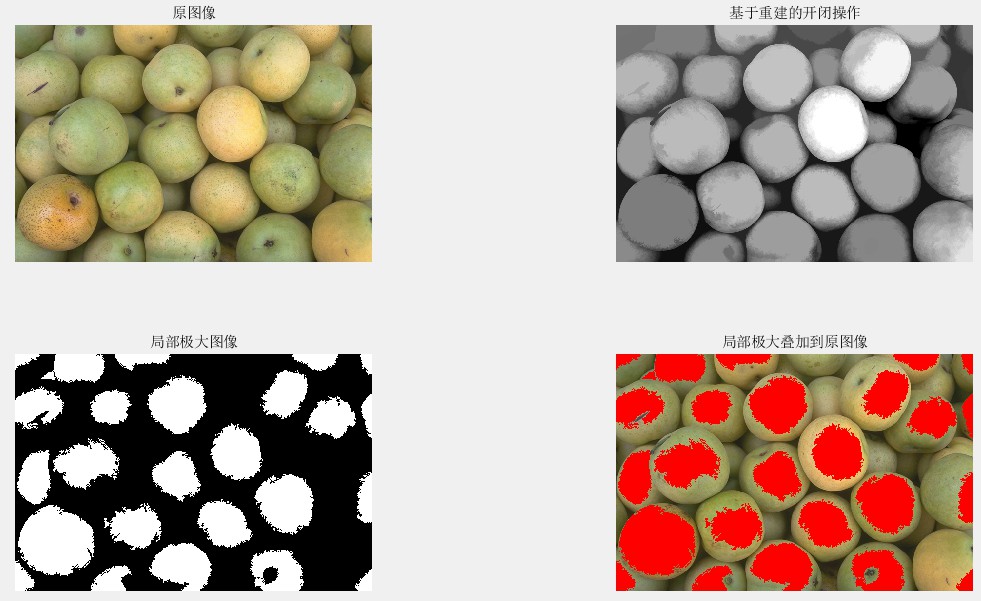
fgm = imregionalmax(Iobrcbr);
figure('units', 'normalized', 'position', [0 0 1 1]);
subplot(1, 3, 1); imshow(I, []); title('灰度图像');
subplot(1, 3, 2); imshow(Iobrcbr, []); title('基于重建的开闭操作');
subplot(1, 3, 3); imshow(fgm, []); title('局部极大图像');
|
1
2
3
4
5
6
7
8
9
|
It1 = rgb(:, :, 1);
It2 = rgb(:, :, 2);
It3 = rgb(:, :, 3);
It1(fgm) = 255; It2(fgm) = 0; It3(fgm) = 0;
I2 = cat(3, It1, It2, It3);
figure('units', 'normalized', 'position', [0 0 1 1]);
subplot(2, 2, 1); imshow(rgb, []); title('原图像');
|
1
2
3
4
5
6
7
8
9
10
|
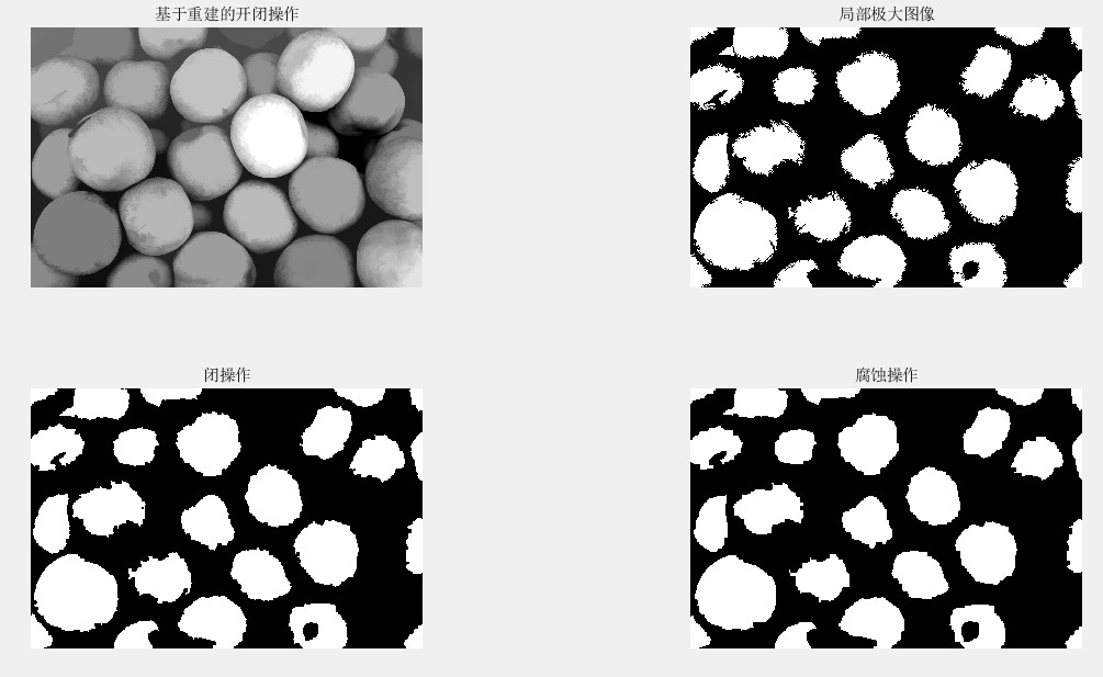
se2 = strel(ones(5,5));
fgm2 = imclose(fgm, se2);
fgm3 = imerode(fgm2, se2);
figure('units', 'normalized', 'position', [0 0 1 1]);
subplot(2, 2, 1); imshow(Iobrcbr, []); title('基于重建的开闭操作');
subplot(2, 2, 2); imshow(fgm, []); title('局部极大图像');
subplot(2, 2, 3); imshow(fgm2, []); title('闭操作');
subplot(2, 2, 4); imshow(fgm3, []); title('腐蚀操作');
|
1
2
3
4
5
6
7
8
9
10
11
12
|
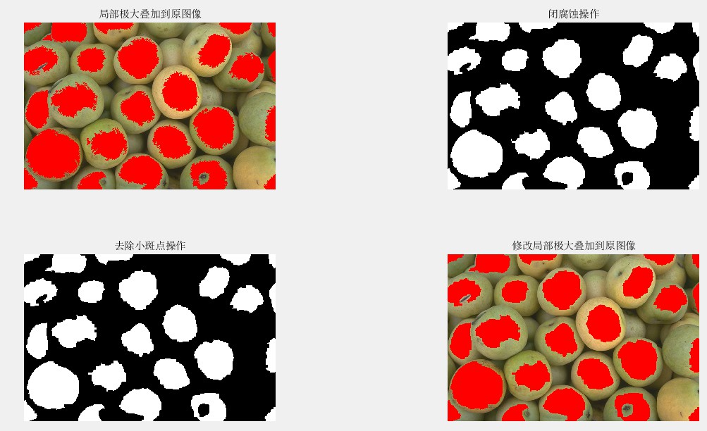
fgm4 = bwareaopen(fgm3, 20);
It1 = rgb(:, :, 1);
It2 = rgb(:, :, 2);
It3 = rgb(:, :, 3);
It1(fgm4) = 255; It2(fgm4) = 0; It3(fgm4) = 0;
I3 = cat(3, It1, It2, It3);
figure('units', 'normalized', 'position', [0 0 1 1]);
subplot(2, 2, 1); imshow(I2, []); title('局部极大叠加到原图像');
subplot(2, 2, 2); imshow(fgm3, []); title('闭腐蚀操作');
subplot(2, 2, 3); imshow(fgm4, []); title('去除小斑点操作');
subplot(2, 2, 4); imshow(I3, []); title('修改局部极大叠加到原图像');
|
1
2
3
4
5
6
|
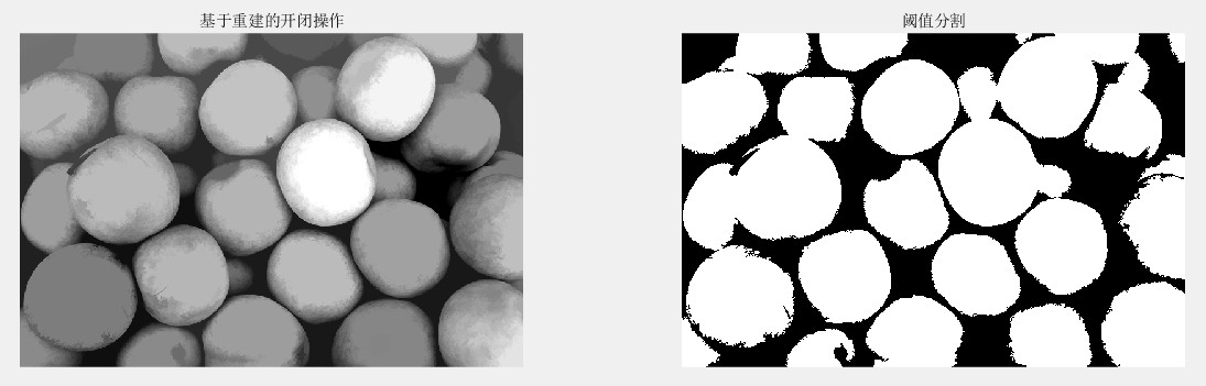
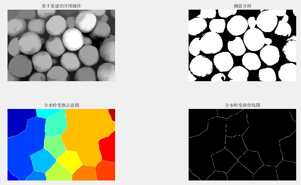
bw = im2bw(Iobrcbr, graythresh(Iobrcbr));
figure('units', 'normalized', 'position', [0 0 1 1]);
subplot(1, 2, 1); imshow(Iobrcbr, []); title('基于重建的开闭操作');
subplot(1, 2, 2); imshow(bw, []); title('阈值分割');
|
1
2
3
4
5
6
7
8
9
|
D = bwdist(bw);
DL = watershed(D);
bgm = DL == 0;
figure('units', 'normalized', 'position', [0 0 1 1]);
subplot(2, 2, 1); imshow(Iobrcbr, []); title('基于重建的开闭操作');
subplot(2, 2, 2); imshow(bw, []); title('阈值分割');
subplot(2, 2, 3); imshow(label2rgb(DL), []); title('分水岭变换示意图');
subplot(2, 2, 4); imshow(bgm, []); title('分水岭变换脊线图');
|
1
2
3
4
5
6
7
|
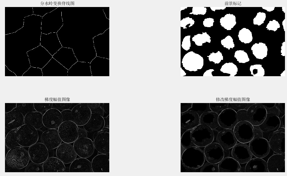
gradmag2 = imimposemin(gradmag, bgm | fgm4);
figure('units', 'normalized', 'position', [0 0 1 1]);
subplot(2, 2, 1); imshow(bgm, []); title('分水岭变换脊线图');
subplot(2, 2, 2); imshow(fgm4, []); title('前景标记');
subplot(2, 2, 3); imshow(gradmag, []); title('梯度幅值图像');
subplot(2, 2, 4); imshow(gradmag2, []); title('修改梯度幅值图像');
|
1
2
3
4
5
6
7
8
9
10
11
12
|
It1 = rgb(:, :, 1);
It2 = rgb(:, :, 2);
It3 = rgb(:, :, 3);
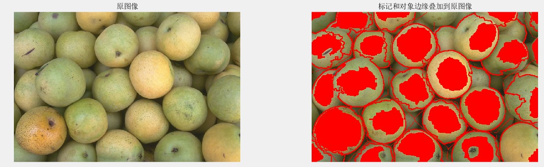
L = watershed(gradmag2);
fgm5 = imdilate(L == 0, ones(3, 3)) | bgm | fgm4;
It1(fgm5) = 255; It2(fgm5) = 0; It3(fgm5) = 0;
I4 = cat(3, It1, It2, It3);
figure('units', 'normalized', 'position', [0 0 1 1]);
subplot(1, 2, 1); imshow(rgb, []); title('原图像');
subplot(1, 2, 2); imshow(I4, []); title('标记和对象边缘叠加到原图像');
|
1
2
3
4
5
6
7
8
9
10
11
12
13
|
Lrgb = label2rgb(L, 'jet', 'w', 'shuffle');
figure('units', 'normalized', 'position', [0 0 1 1]);
subplot(1, 2, 1); imshow(rgb, []); title('原图像');
subplot(1, 2, 2); imshow(Lrgb); title('彩色分水岭标记矩阵');
figure('units', 'normalized', 'position', [0 0 1 1]);
subplot(1, 2, 1); imshow(rgb, []); title('原图像');
subplot(1, 2, 2); imshow(rgb, []); hold on;
himage = imshow(Lrgb);
set(himage, 'AlphaData', 0.3);
title('标记矩阵叠加到原图像');
|
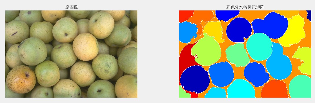
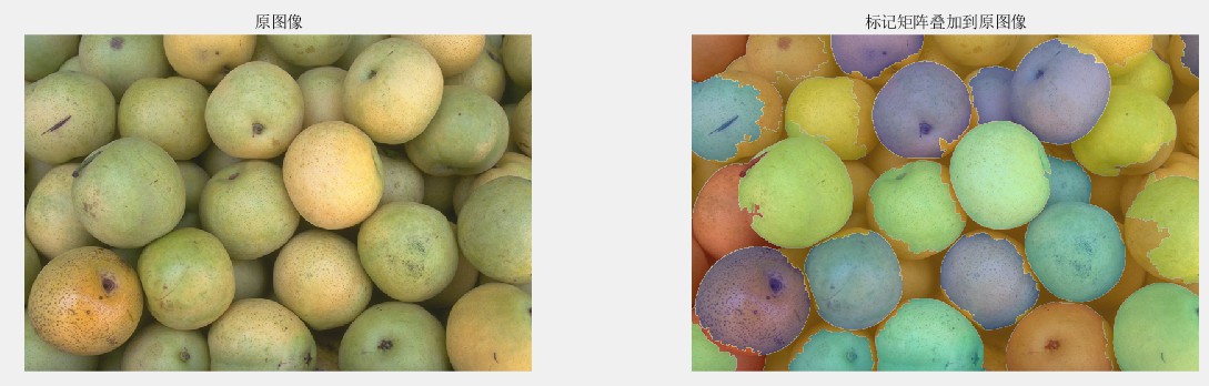
使用分水岭算法应对图像目标区域沾连分割问题,常能达到意象不到的效果。
内容参考: